Simulated Tape and Universal Behavior

Having spent a lot of time solving equations related to sticky tape models, including trying to work solutions in my head while driving to Grandma and Grandpa's with the kids, and making some measurements of real tapes, there was only one thing left to do: try simulating this problem in VPython. Because I'm a physics nerd who knows just enough about programming to be dangerous...

Finding the full solution to the real sticky tape scenario is kind of a miserable process, because it involves a long continuous tape with charge all down its length, which is kind of complicated, and then there's a bunch of trigonometry to get the forces. The equations are slightly easier to set up if you think in terms of energy, but you still wind up trying to find the roots of an equation with a couple of different trig functions, and that's a huge hassle.

The basic physics involved is really simple, though, so it's very easy to write a program that includes all the relevant forces, and let it find the equilibrium position for you. So that's what I tried to do.

The Model/p>

Screen shot of the "tape" simulation.

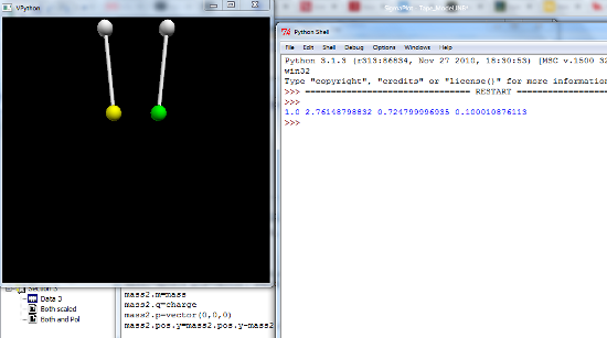
The long charged tape thing is till a problem, so I opted to simplify things by treating them as point charges hanging from strings. This makes the set-up vastly easier to put into VPython, and you can see a screen shot of the result above.

The goal here was to keep things as simple as possible, so I started them out hanging straight down at the pivot points, which were separated by a fixed distance in the 10-50 cm sort of range, comparable to what I used when I was playing with actual tapes. The simulation includes the electrostatic force between the charged balls, a gravitational force from the mass (300 mg, comparable to the tapes used in lab), and a tension force from the string, which I modeled as a spring, as in the simulated pendulum investigations last year. I start the string with the appropriate stretch to minimize oscillations along the string. I made a token effort to do the tension force analytically, but then decided that was annoying, and went back to the spring thing that worked in the past.

Of course, if you just released these from rest, you would see them oscillate wildly back and forth, so I added a viscous drag force to the simulation. Doing that reduces the velocity of the moving balls, causing them to settle down toward the equalibrium point where the force is zero. The value of the drag coefficient was pretty much randomly chosen, a value that seemed to work reasonably well. I ran the simulations for five seconds of simulated time, and if the system was going to reach equilibrium, it generally did so very quickly, within a few seconds. In the same way, a system past the tipping point where the "tapes" fly up and stick to each other generally did so within a second or two.

The process from there was very simple: I rean the simulation lots and lots of times, changing the initial separation. If the system reached an equilibrium position, I recorded the value of the final separation between balls as a function of the initial separation. Then I tried to find the smallest possible starting separation where the system found a stable equilibrium.

If you're familiar with VPython, or would like to play around with the code for this simulation, it's posted on gist, so you can laugh at my rudimentary coding abilities.

The Results

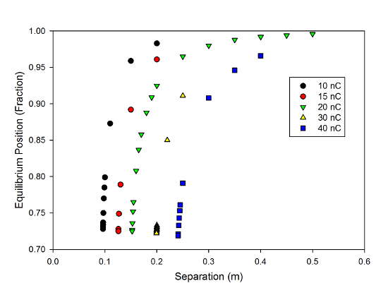
The results, for several different values of the charge on the "tape" look like this:

Final position vs. starting separation for the "tape" model, showing the tipping point behavior.

You can very clearly see the "tipping point" behavior here-- for each charge, the tapes are basically unmoved at large initial separation, but the final separation falls off a cliff as you come in closer. This follows the general pattern you expect, too: tapes with smaller total charge have smaller values of the tipping point, while tapes with bigger charges are only stable for larger initial separations.

All of these curves have a very similar shape, which suggests another physicist-y trick, namely a check for universal scaling. When I did the original sticky tape toy model, I found it useful to go to dimensonless variables. In a similar way, the shape of these curves suggests that there may be a very general phenomenon at work, here, so I scaled the horizontal axis for all these curves to put it in terms of the minimum separation I measured. So, for example, with a charge of 20 nanocoulombs, the smallest separation I measured a stable equilibrium for was 0.1523 m, so I divided all the separation values by 0.1523, creating a new dimensionless parameter that is the separation as a multiple of the minimum stable point.

Why do that? Because it let me make this graph:

Final position vs. initial separation for the "tape" simulation, scaled to the tipping point, showing the universal behavior.

This shows the same data from the previous plot, but with the horizontal axis scaled. And you can see right away, all of the data fall on a single universal curve, indicating that there's a very general thing going on here. If you bump up the charge by some amount, you can just multiply all the distances you're working with by the appropriate factor, and get exactly the same behavior.

This is the sort of graph that warms the hearts of physicists who make them. If you can figure out a way to make all your data from a bunch of different conditions-- whether real experimental points or numerical simulations-- fall onto a single curve, that means you've got a good handle on the essentials of the situation. So, this made me very happy. I don't know exactly what the shape of that curve is, mind, but the fact that everything fits the same shape is really nice.

The Toy Model

Of course, what got me off on this was a study of this where I replaced the hanging tapes with a ball-on-a-spring model, because that system allowed me to work with simpler equations and get some numerical answers. That might have seemed a little dubious, so what happens if I look at that toy model in VPython?

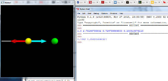
Well, I can do that easily enough-- more easily than the pendulum version, actually, and it looks like this:

The toy model version, representing the system by a mass on a spring.

I used the same charges and mass as in the pendulum simulation, and set the spring constant to be close to make the key ratio from that earlier calculation close to the magic value of 4/27 for a separation of around 10cm. There obviously wasn't any need for gravity in this case, but I kept the drag force trick. The code for this one is here, if you want to play with it.

In this case, I did the same sort of run, looking for the smallest initial separation that gave a stable equilibrium, though here I wrote down the final stretch of the spring as a fraction of the initial separation, so the values increase rather than decrease. You still see very similar "tipping point" behavior, though:

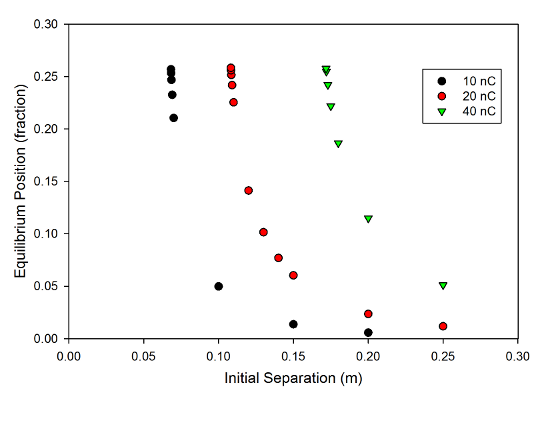Data for the toy model version of the system, showing the equilibrium position as a function of initial separation.

And just as with the pendulum model, these can be re-scaled on the horizontal axis so that they all fall on a single universal curve:

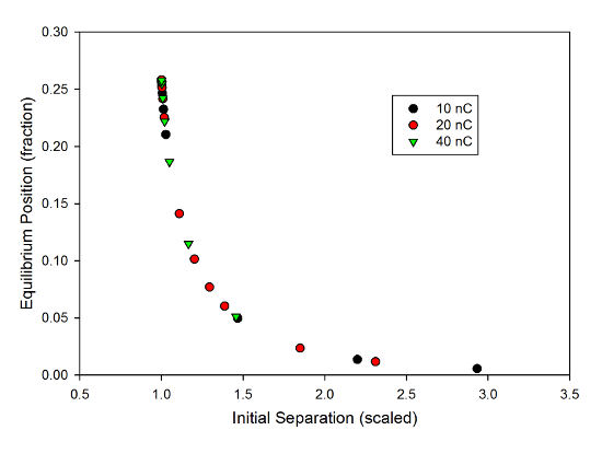The toy model data, scaled to the minimum separation for each charge, showing the universal behavior.

So, while the scenario is much simpler to describe mathematically, you can see that the "toy model" version indeed captures the essential physics. In both cases, you see a nice, clean universal behavior for a bunch of different charges.

But what's really cool is what happens when you re-calculate the vertical axis values, as well. The fractional position for the toy model is easily converted to a fractional separation, comparable to what I recorded for the pendulum data, and if we plot the data from both models together, this is what we get:

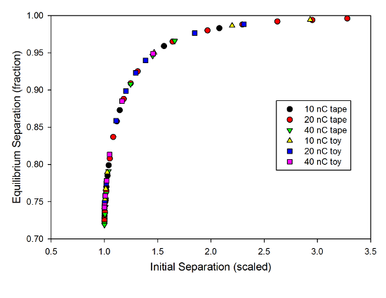Comparison of the two different simulations, scaled to the "tipping point" showing the universal behavior.

that plot includes data from both the "toy model" version and the somewhat more realistic pendulum version. And if you can see a difference between them, your eye is keener than mine. All of the data, from both models, follow exactly the same curve, showing that the toy model really captures all of the essential behavior of the system-- captures it basically perfectly, in fact. This is not something that will really surprise experienced physicists-- basically anything interesting can be modeled as a mass on a spring in some limit-- but it's nice to see such a clear demonstration of it. And hopefully, this can help convince you that when we play our spherical cow games, we're not just talking out our asses.

Now, there are still a few other aspects of this to explore. If you look closely at the numbers on the unscaled graphs, you might find a discrepancy between the simulation results and the numerical values discussed in that first sticky tape post. There's a good reason for this, having to do with the way I set up the simulations, but for now, I'll just tease you with that statement, and save the full explanation for a later post. There's also the question of the atomic polarizability measurement and whether I can provide any validation of that. So we're not done with sticky tape and VPython quite yet...